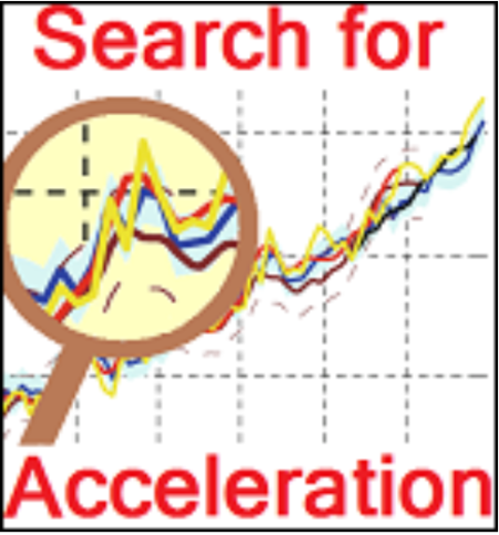
The Search for Acceleration: Table of Contents and Introduction

Church and White 2011 figure 6 with my annotation.

Introduction

The most commonly quoted 20th century sea level data derived from tide gauges has the average rise rate at about 1.8 mm per year, but the satellite data since 1993 has the rise rate at about 3 mm per year.  I have always wondered if those two facts could be reconciled. If they are both true, does that mean there has been an extreme acceleration in sea level rise rates at the tail end of the 20th century? Shouldn’t such an acceleration be apparent in the tide gauge data? So I have spent much time recently searching the data for such an acceleration.

.

Satellite data – University of Colorado

For all my searching, the outcome is still somewhat ambiguous. This is a series of posts on that search.

Local, Regional and Global

I will frequently refer to “local,” “regional” and “global” sea level rise rates.  The global sea level rise rate is what makes the news these days, and its meaning is seemingly obvious.  

When I talk about a local sea level rise rate, I will be referring to data from a single tide gauge station. A “region” will be a group of tide gauge stations with some geographical properties in common and some coherence in their sea level data.  A regional sea level rise rate will be derived from a weighted average of data form tide gauges in the same region. 

Acceleration, not rise rate

My goal is not to establish any global or local sea level rise rates, but rather to look for evidence of a large acceleration at the end of the 20th century.  In some ways, finding the acceleration is easier than finding the rise rate.  

As shown in the first post, two tide gauge stations in the same region may have very different long term rise rates, but when detrended have very similar shorter term features.  In this case the long term rise rates are obviously dominated by some different local geological phenomena, while the shorter term features are governed by regional or global phenomena.  Detrending the local tide gauge data abandons any possibility of finding “true” rise rates, but it does not affect the acceleration information in the data.

Typically, I will not actually plot the acceleration data, but rather the “relative” sea level rise rate from derived from the detrended sea level data.  Readers can visually spot the periods of acceleration and periods of relatively high or low rise rates.

Another advantage of detrending 

When I detrend data it will be over some time period largely covered by all of the regional data sets.  However, some of those data sets may also cover other time periods.  If the regional data sets were averaged (weighted or not) without first detrending, then those time periods not covered by all the data sets will have rise rates dominated by the local effects of the data sets that do cover them.  This problem is largely mitigated by detrending.

Table of Contents

Here is a one line summary of the posts in this series.  This page and summary will be updated each time a new post is added to the series.

Part 1.  Background information

Part 2.  East Coast of North America.

Part 3.  Japan

Part 4.  Mea Culpa – Mistakes in Parts 1 & 2 are explained and corrected

Part 5.  The Netherlands

Part 6.  Australia.  My standard analysis plus relative sea level rise rate orthogonal to ENSO3.4

Part 7.  West coast of North America.  Standard analysis and ENSO3.4.

Part 8. Hawaii. Standard analysis and ENSO3.4.

Part 9. Baltic Sea. Standard anlysis.

Part 10. US Gulf Coast. Standard analyis

This page and summary will be updated each time a new post is added to the series.